
| 일 | 월 | 화 | 수 | 목 | 금 | 토 |
|---|---|---|---|---|---|---|
| 1 | 2 | 3 | ||||
| 4 | 5 | 6 | 7 | 8 | 9 | 10 |
| 11 | 12 | 13 | 14 | 15 | 16 | 17 |
| 18 | 19 | 20 | 21 | 22 | 23 | 24 |
| 25 | 26 | 27 | 28 | 29 | 30 | 31 |
- Cypher
- Graph Ecosystem
- TigerGraph
- 그래프 에코시스템
- DeepLearning
- 분산 병렬 처리
- 딥러닝
- SQL
- SparkML
- r
- Python
- BigData
- 그래프
- spark
- Neo4j
- TensorFlow
- GSQL
- RStudio
- Graph Tech
- 그래프 데이터베이스
- graph
- 빅데이터
- Federated Learning
- 그래프 질의언어
- 인공지능
- graph database
- GDB
- RDD
- GraphX
- 연합학습
- Today
- Total
Hee'World
기상데이터를 이용한 Shiny App구현 본문
기상데이터를 이용하여 데이터를 확인해 볼 수 있는 기본적인 Shiny앱을 구현합니다.
아래와 같은 탭형식의 기상데이터 탐색을 Shiny로 구현한 화면입니다.

사용환경 : Windows 10, R3.5, RStudio 1.1463
R 주요 패키지 : Shiny, ggplot2, DT, rpart, corrplot
먼저 기상데이터를 수집하기 위해서는 기상청에서 운영하는 "날씨마루"와 "기상자료개방포털"를 활용하여 획득 할 수 있습니다.
https://bd.kma.go.kr/kma2019/svc/main.do
기상청 날씨마루 - 기상 빅데이터 분석 플랫폼 및 기상융합서비스
bd.kma.go.kr
https://data.kma.go.kr/cmmn/main.do
기상자료개방포털
data.kma.go.kr
필자는 기상자료개방포털에서 데이터를 수집하였으며, 다운로드하는 방법은 어렵지 않기 때문에 다루지 않겠습니다.
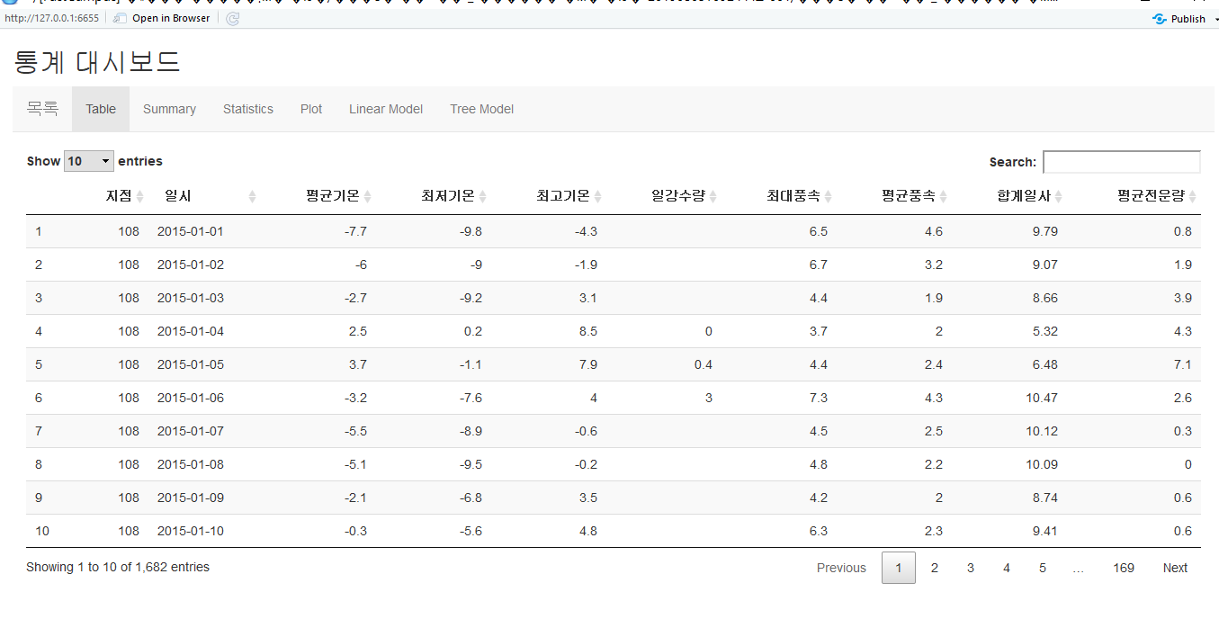
서울지점(108)의 2015년 08월 ~ 2019년 08월 중 평균기온, 최저기온, 최고기온, 일강수량, 최대 풍속, 평균 풍속, 합계 일사, 평균 전운량을 선택하여 다운로드 하였습니다.
<서울지점 기상데이터>

데이터준비가 완료되었으면, R을 이용하여 Shiny App을 구현합니다.
1. 데이터를 로드하고, 날짜형으로 변환합니다.
# 데이터 로드
weather_data <- read.csv("C:/Users/jonghee/Documents/20190810131821.csv", header = T)
names(weather_data) <- c("지점","일시","평균기온","최저기온","최고기온","일강수량","최대풍속","평균풍속","합계일사","평균전운량")
head(weather_data)
str(weather_data)

# 날짜형식 변환
weather_data$일시 <- as.Date(weather_data$일시)
2. Shiny의 UI 부분을 작성합니다.
ui <- fluidPage(
  titlePanel("통계 대시보드"),
  navbarPage("목록",
                 tabPanel("Table",
                      DT::dataTableOutput("table")
                 ),
                 tabPanel("Summary",
                      verbatimTextOutput("summary"),
                      verbatimTextOutput("str")
                 ),
                 tabPanel("Statistics",
                          sidebarLayout(
                            sidebarPanel(
        .....................................
3. Shiny의 UI에서 선택 또는 입력받은 데이터를 처리하는 server 부분을 작성합니다.
server <- function(input, output, session) {
selectedData <- reactive({
weather_data[, c(input$xcol, input$ycol)]
})
output$table <- DT::renderDataTable({
DT::datatable(weather_data)
})
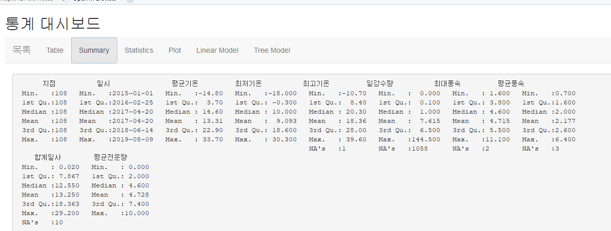
output$summary <- renderPrint({
summary(weather_data)
})
output$str <- renderPrint({
str(weather_data)
})
...............................
4. 작성된 ui와 server를 shinyApp 함수로 실행하면 아래와 같은 화면이 실행됩니다.
shinyApp(ui=ui, server=server)
<기술통계량>
<상관계수 및 시각화>

<기본 차트>

<Tree Model>

지금까지 간단하게 기상데이터를 이용하여 Shiny App을 구현하였는데, 실제로는 더 다양한 프레임워크와 함께 윈도우환경이 아닌 서버환경에서 구현되어 활용되고 있습니다.
그리고, Shiny 공식 홈페이지에서 Gallery 메뉴를 참고하면 더 많은 레퍼런스와 사례를 확인 할 수 있습니다.
https://shiny.rstudio.com/gallery/
Shiny - Gallery
shiny.rstudio.com
전체 코드 및 데이터
############### Shiny ######################

#install.packages("shiny")
#install.packages("ggplot2")
#install.packages("markdown")
#install.packages("DT")
#install.packages("corrplot")
#install.packages(c("rpart", "rpart.plot"))

library(shiny)
library(ggplot2)
library(DT)
library(markdown)
library(rpart)
library(rpart.plot)
library(corrplot)

##########################################################

weather_data <- read.csv("C:/Users/jonghee/Documents/20190810131821.csv", header = T)
names(weather_data) <- c("지점","일시","평균기온","최저기온","최고기온","일강수량","최대풍속","평균풍속","합계일사","평균전운량")
head(weather_data)
str(weather_data)
weather_data$일시 <- as.Date(weather_data$일시)

ui <- fluidPage(
  titlePanel("통계 대시보드"),
  navbarPage("목록",
                 tabPanel("Table",
                      DT::dataTableOutput("table")
                 ),
                 tabPanel("Summary",
                      verbatimTextOutput("summary"),
                      verbatimTextOutput("str")
                 ),
                 tabPanel("Statistics",
                          sidebarLayout(
                            sidebarPanel(
                              selectInput('xcol', 'X Variable', names(weather_data)),
                              selectInput('ycol', 'Y Variable', names(weather_data),
                                          selected=names(weather_data)[[2]])
                            ),
                            mainPanel(
                              verbatimTextOutput("cor"),
                              plotOutput("corrplot"),
                              verbatimTextOutput("totalcorr")
                            )
                          )
                 ),
                 tabPanel("Plot",
                          sidebarLayout(
                            sidebarPanel(
                              radioButtons("plotType", "Plot type",
                                           c("Scatter"="p", "Line"="l", "BoxPlot"="b", "BarPlot"="bp")
                              )
                            ),
                            mainPanel(
                              plotOutput("plot")
                            )
                          )
                 ),
                 tabPanel("Linear Model",
                          mainPanel(
                            verbatimTextOutput("lm"),
                            plotOutput("lmplot")
                          )

                ),
                 tabPanel("Tree Model",
                      mainPanel(
                        verbatimTextOutput("tree"),
                        plotOutput("treeplot")
                      )

                 )

  )
)

#server <- function(input, output){

  selectedData<-reactive({
    get(input$dataSelect)
  })

  weather_data2 = weather_data[sample(nrow(weather_data), 1000), ]
  output$mytable1 <- DT::renderDataTable({
    DT::datatable(weather_data2[, input$show_vars, drop = FALSE])
  })

  #output$out1 <- renderPrint({
  #  summary(selectedData())
  #})
  #output$out2 <- renderPrint({
  #  str(selectedData())
  #})
  #output$out3 <- renderPlot({
  #  plot(selectedData())
  #})
}

server <- function(input, output, session) {

  selectedData <- reactive({
    weather_data[, c(input$xcol, input$ycol)]
  })

  output$table <- DT::renderDataTable({
    DT::datatable(weather_data)
  })

  output$summary <- renderPrint({
    summary(weather_data)
  })

  output$str <- renderPrint({
    str(weather_data)
  })

  output$cor <- renderPrint({
    cor(selectedData(), use="complete.obs")
  })

  output$corrplot <- renderPlot({
    corrplot(cor(weather_data[,3:10], use="complete.obs"))
  })

  output$totalcorr <- renderPrint({
    cor(weather_data[,3:10], use="complete.obs")
  })

  output$plot <- renderPlot({
    # plot(weather_data, type=input$plotType)
    if(input$plotType == "p"){
      plot(weather_data)
    }
    else if(input$plotType == "l"){
      ggplot(weather_data, aes(x=일시, y=평균기온)) + geom_line()
    }
    else if(input$plotType == "b"){

      ggplot(weather_data, aes(x=지점, y=평균기온)) + geom_boxplot()
      ggplot(weather_data, aes(x=지점, y=평균전운량)) + geom_boxplot()
    }
    else if(input$plotType == "bp"){
      ggplot(weather_data, aes(x=최저기온, y=평균기온)) + geom_bar()
    }
  })

  output$lm <- renderPrint({
    summary(lm(평균기온 ~ 최저기온 + 최고기온 + 일강수량 + 최대풍속 + 평균풍속 + 합계일사 + 평균전운량, data=weather_data))
  })

  output$lmplot <- renderPlot({
    plot(lm(평균기온 ~ 최저기온 + 최고기온 + 일강수량 + 최대풍속 + 평균풍속 + 합계일사 + 평균전운량, data=weather_data))
  })

  output$tree <- renderPrint({
    rpart(평균기온 ~ 최저기온 + 최고기온 + 일강수량 + 최대풍속 + 평균풍속 + 합계일사 + 평균전운량, data=weather_data)
  })

  output$treeplot <- renderPlot({
    rpart.plot(rpart(평균기온 ~ 최저기온 + 최고기온 + 일강수량 + 최대풍속 + 평균풍속 + 합계일사 + 평균전운량, data=weather_data))
  })
}


shinyApp(ui=ui, server=server)
기상데이터
'Programming > R' 카테고리의 다른 글
| R 버전 업데이트 (0) | 2021.12.11 |
|---|---|
| Tensorflow_R_MNIST 예제 (Keras) (0) | 2020.04.13 |
| tensorflow in r 설치 (0) | 2017.07.19 |
| Sparklyr 설치 (0) | 2017.07.19 |
| kNN 알고리즘 (0) | 2015.05.03 |


